PV Power Plant

Tip

PV power plant is modelled as a two-stage inverter with the first stage being the boost DC-DC converter, and the second stage being the voltage source inverter. At the output of the VSC is attached an LCL filter.

Mathematical Modeling

The PV array is taken as an aggregated model of the entire plant, see Fig. Figure 1.

Figure 1: Two-stage PV inverter with LCL filter, image taken from Zhao et al. (2022).

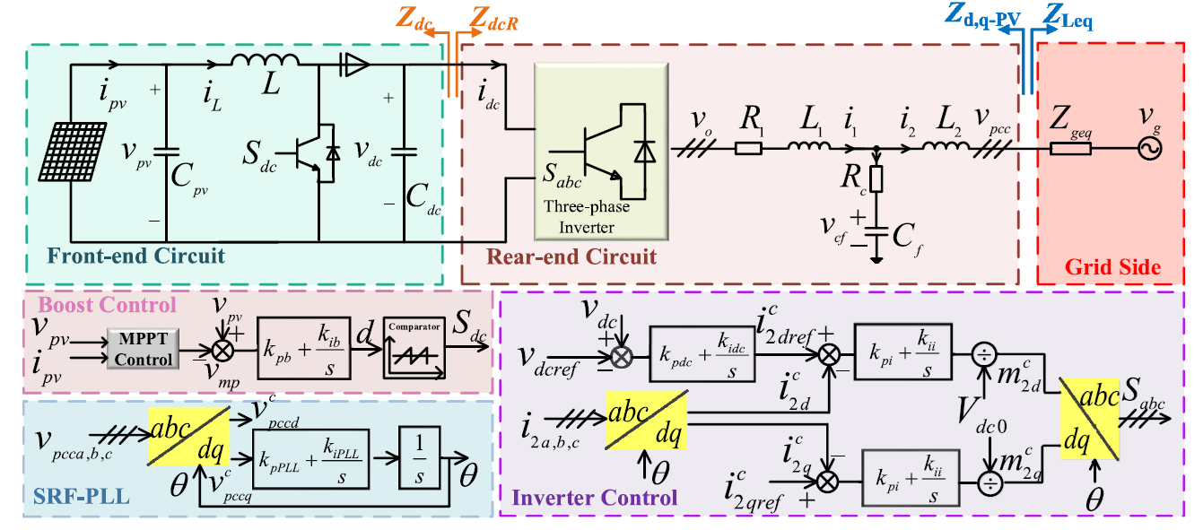
To estimate the operating point of the boost converter and the VSC, we follow the averaged model described in Wen et al. (2014) and Khazaei, Tu, and Liu (2020), with known PV current and power, \(V_{pcc}\), and assuming ideal PLL operation.

\[\begin{equation} V_{pv} = \frac{P_{pv}}{I_{pv}}, \quad I_{dc} = \frac{P_{pv}}{V_{dc}}, \quad D = 1 - \frac{V_{pv}}{V_{dc}} \end{equation}\]

\[\begin{equation} V_{pccd} = V_{pcc}, \sqrt{\frac{2}{3}} \quad V_{pccq} = 0 \end{equation}\]

\[\begin{equation} I_{2d} \approx \frac{2 P_{pv}}{3 V_{pccd}}, \quad I_{2q} \approx \frac{2 Q}{3 V_{pccd}} \end{equation}\]

\[\begin{equation} V_{Cf,dq} = \frac{ V_{pcc,dq} \pm \omega R_c C_f V_{pcc,qd} \mp \omega L_2 I_{2,qd} + \omega^2 R_c C_f L_2 I_{2,dq} }{ 1 + (\omega R_c C_f)^2 } \end{equation}\]

\[\begin{equation} I_{1,dq} = I_{2,dq} \mp \omega C_f V_{Cf,qd} \end{equation}\]

\[\begin{equation} V_{o,dq} = V_{pcc,dq} - R_1 I_{1,dq} \mp \omega L_1 I_{1,qd} - R_2 I_{2,dq} \mp \omega L_2 I_{2,qd} \end{equation}\]

\[\begin{equation} M_{dq} = \frac{2 V_{o,dq}}{V_{dc}} \end{equation}\]

Based on Fig. Figure 1, a small-signal model can be constructed as described in Wen et al. (2014) and Zhao et al. (2022), and is depicted in Fig. Figure 2.

Figure 2: Small-signal model in the dq-frame for the two-stage PV inverter shown in Fig. Figure 1, image taken from Zhao et al. (2022).

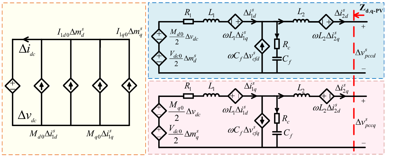
Based on this model, the transfer functions between the inputs \(\Delta m^s_{dq}\), \(\Delta i^s_{2,dq}\), and \(\Delta v_{dc}\), and the outputs \(v^s_{pcc,dq}\) and \(i_{dc}\) can be formulated as follows Zhao et al. (2022):

\[\begin{equation} \begin{bmatrix} \Delta i_{dc} \\ 0 \end{bmatrix} = \underbrace{ \left( N_m Y_C (Z_{RL1} Y_C + I)^{-1} Z_{L2} + N_m \right) }_{G_{ii}} \begin{bmatrix} \Delta i^s_{2d} \\ \Delta i^s_{2q} \end{bmatrix} + \underbrace{ \left( N_m Y_C (Z_{RL1} Y_C + I)^{-1} \right) }_{G_{vi}} \begin{bmatrix} \Delta v^s_{pccd} \\ \Delta v^s_{pccq} \end{bmatrix} + \underbrace{ N_i }_{G_{mi}} \begin{bmatrix} \Delta m^s_d \\ \Delta m^s_q \end{bmatrix} \end{equation}\]

\[\begin{equation} \begin{bmatrix} \Delta v^s_{pccd} \\ \Delta v^s_{pccq} \end{bmatrix} = \underbrace{ - H_1^{-1} ( H_1 Z_{L2} + Z_{RL1} ) }_{G_{iv}} \begin{bmatrix} \Delta i^s_{2d} \\ \Delta i^s_{2q} \end{bmatrix} + \underbrace{ ( H_1^{-1} H_m ) }_{G_{vv}} \begin{bmatrix} \Delta v_{dc} \\ 0 \end{bmatrix} + \underbrace{ ( H_1^{-1} H_v ) }_{G_{mv}} \begin{bmatrix} \Delta m^s_d \\ \Delta m^s_q \end{bmatrix} \end{equation}\]

for \(H_1 = Z_{RL1} Y_C (Z_{R_C} Y_C + I)^{-1} + I\), \(N_m = \begin{bmatrix} M_d & M_q \\ 0 & 0 \end{bmatrix}\), \(N_i = \begin{bmatrix} I_{1d} & I_{1q} \\ 0 & 0 \end{bmatrix}\), \(H_m = \begin{bmatrix} M_d/2 & 0 \\ M_q/2 & 0\end{bmatrix}\), \(H_v = \begin{bmatrix} V_{dc}/2 & 0 \\ 0 & V_{dc}/2 \end{bmatrix}\), \(Z_{RL1} = \begin{bmatrix} R_1+sL_1 & -\omega L_1 \\ \omega L_1 & R_1 + sL_1 \end{bmatrix}\), \(Z_{R_C} = \begin{bmatrix} R_C & 0 \\ 0 & R_C \end{bmatrix}\), \(Z_{L2} = \begin{bmatrix} sL_2 & -\omega L_2 \\ \omega L_2 & sL_2 \end{bmatrix}\), and \(I\) is an identity matrix of size \(2 \times 2\).

The controlling loops influence the system with the introduction of matrices:

• DC voltage control: \(i^c_{2d, ref} = g_{dc} (v_{dc} - v_{dc, ref})\), \(g_{dc} = k_{pdc} + \frac{k_{idc}}{s}\), and \(G_{dc} = \begin{bmatrix} g_{dc} & 0 \\ 0 & 0 \end{bmatrix}\);
• Current control: \(i^c_{2d, ref} = g_{dc} (v_{dc} - v_{dc, ref})\), \(g_{dc} = k_{pdc} + \frac{k_{idc}}{s}\), and \(G_{dc} = \begin{bmatrix} g_{dc} & 0 \\ 0 & 0 \end{bmatrix}\);
• PLL: \(H_{PLL} = k_{ppll} + \frac{k_{ipll}}{s}\), and \(G_{PLL} = \frac{H_{PLL}}{s + V_{pccd} H_{PLL}}\), \[ m^c_{dq} = m^s_{dq} + \underbrace{\begin{bmatrix} 0 & G_{PLL} M_q \\ 0 & -G_{PLL} M_d \end{bmatrix}}_{G_{PLLM}} \, v^s_{pcc,dq}, \qquad i^c_{2dq} = i^s_{2dq} + \underbrace{\begin{bmatrix} 0 & G_{PLL} I_{2q} \\ 0 & -G_{PLL} I_{2d} \end{bmatrix}}_{G_{PLLI}} \, v^s_{pcc,dq}. \]

Influence of the PV module and boost converter, and controller is given through the impedance \(Z_{dc}\): \[\begin{equation} z_{dc} = \frac{sL(sC_{pv}-k_{pv}) + 1 + g_B V_{dc} (1-\lambda)}{(1-D)^2 (k_{pv} - sC_{pv}) + (D-1) g_B I_{L} (1-\lambda) -sC_{dc} - sC_{dc} V_{dc} g_B (1-\lambda) + s^2 LC_{dc} (k_{pv} - sC_{pv})}, \end{equation}\] where \[\begin{align*} k_{pv} = -\frac{q (N_p I_0 + N_p I_{sc} - I_{pv})}{nkT N_s}, \\ k_{mp} = \frac{(nkTN_s / q)^2}{I_0N_pV_{mp} \exp(qV_{pv}/(nkTN_s)) + \frac{I_{pv}}{V_{mp}} (nkTN_s/q)^2}, \\ \lambda = k_{pv} k_{mp}, \qquad g_B = k_{pB} + \frac{k_{iB}}{s}, \end{align*}\]

where \(N_s\) and \(N_p\) are the numbers of series and parallel connected PV panels, respectively, \(I_0\) is the diode saturation current under normal conditions, \(I_{sc}\) is the short current of PV cell under the standard condition, \(T\) is the temperature (taken as \(T = T_n = 298.18 \text{ K}\)), \(k = 1.38062 \times 10^{-23} \text{ J/K}\) is the Boltzmann’s constant, \(q = 1.60217 \times 10^{-23} \text{ C}\) is the unit electric charge.

Finally, dq-impedance is calculated as:

\[\begin{equation} Z_{PV} = -\left( J_A F_A^{-1} F_B + J_B \right) \left( J_C - J_A F_A^{-1} F_C \right)^{-1} \end{equation}\]

\[\begin{equation} J_A = G_{vv} + G_{mv} G_v G_i G_{dc} \end{equation}\]

\[\begin{equation} J_B = G_{iv} - G_{mv} G_v G_i \end{equation}\]

\[\begin{equation} J_C = G_{mv} \left( G_v G_i G_{PLLI} + G_{PLLM} \right) + I \end{equation}\]

\[\begin{equation} F_A = I - Z_{dc} G_{mi} G_v G_i G_{dc} \end{equation}\]

\[\begin{equation} F_B = Z_{dc} G_{ii} - Z_{dc} G_{mi} G_v G_i \end{equation}\]

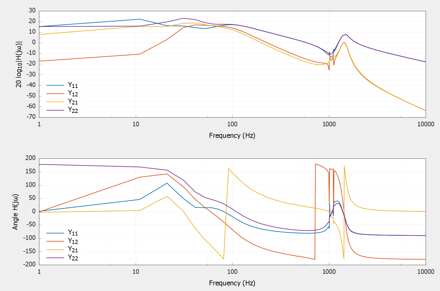
The results of the code execution in Harmony are available in Figure 3. The parameters used for simulation are:

• PV module: \(N_p = 720\), \(N_s = 2760\), \(n = 1.5\), \(I_{sc} = 2.5 \text{ A}\), \(I_0 = 10^{-10} \text{ A}\), \(C_{pv} = 7.2 \text{ mF}\), \(I_{pv} = 6570 \text{ A}\), \(P_{pv} = 2.8 \text{ MW}\);
• Boost converter: \(L = 16 \, \mu \text{H}\), \(C_{dc} = 70 \text{ mF}\), \(V_{dc} = 900 \text{ V}\), \(k_{pB} = 4.9809 \times 10^{-6}\), \(k_{iB} = 4.9809 \times 10^{-9}\);
• LCL filter: \(L_1 = 103 \, \mu \text{H}\), \(C_f = 220 \, \mu \text{F}\), \(L_2 = 125 \, \mu \text{H}\), \(R_1 = 0\), \(R_C = 0.1 \, \Omega\);
• PCC: \(V_{g, rms} = 690 \text{ V}\), \(f_g = 50 \text{ Hz}\);
• VSC: current control - \(k_{pi} = 0.45\), and \(k_{ii} = 69.7\), DC voltage control - \(k_{pdc} = 1\), and \(k_{idc} = 500\), PLL - \(k_{ppll} = 0.5\), and \(k_{ipll} = 1\).

Figure 3: Bode plots of the dq admittance for the PV inverter.

Code Explanation

For detailed code information, see the Harmony manual.

References

Khazaei, Javad, Zhenghong Tu, and Wenxin Liu. 2020. “Small-Signal Modeling and Analysis of Virtual Inertia-Based PV Systems.” IEEE Transactions on Energy Conversion 35 (2): 1129–38.

Wen, Bo, Dushan Boroyevich, Rolando Burgos, Paolo Mattavelli, and Zhiyu Shen. 2014. “Small-Signal Stability Analysis of Three-Phase AC Systems in the Presence of Constant Power Loads Based on Measured Dq Frame Impedances.” IEEE Transactions on Power Electronics 30 (10): 5952–63.

Zhao, Ensheng, Yang Han, Xiangyang Lin, Ping Yang, Frede Blaabjerg, and Amr S Zalhaf. 2022. “Impedance Characteristics Investigation and Oscillation Stability Analysis for Two-Stage PV Inverter Under Weak Grid Condition.” Electric Power Systems Research 209: 108053.