Wind Turbine Type-3
Type-III wind turbines (WT3), also known as DFIG-based turbines, are widely used in grid-connected wind power plants. In this configuration, the generator stator is directly connected to the grid, while the rotor is interfaced through a back-to-back converter, enabling variable-speed operation and flexible active and reactive power control. WT3 turbines are typically connected to the grid via a medium-voltage collector system and a substation transformer.
Mathematical Modeling
The type-III WTs are shown in Figure 1. A type-III wind turbine feeds the grid side through a back-to-back converter. The wind turbine is connected to the MV bus through transformer \(T_1\). The current flowing to the MV bus is scaled by \(N_t\), representing that a single wind turbine is equivalent to \(N_t\) wind turbines connected in parallel Guest, Jensen, and Rasmussen (2020). A capacitor \(C\), representing the shunt capacitance of the cable collector, is connected to the MV bus. The MV bus is connected to the PCC through a substation (SS) transformer \(T_2\). The PCC is connected to the grid through the cables.
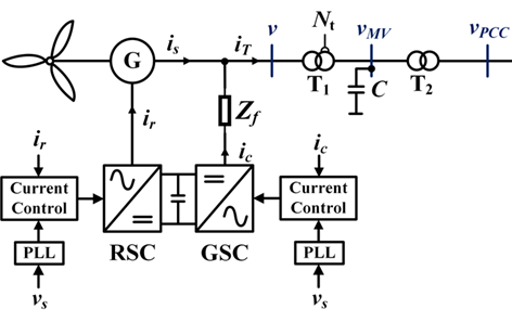
The RSC and GSC are controlled by the current controllers implemented at the d-q domain. Since the outer control loops to generate current references operate much more slowly than the inner current loops, the dynamics of these outer loops can be ignored Vieto and Sun (2018). In this sense, the equivalent harmonic impedance model can be developed in Figure 2.
In Figure 2, the grid background harmonics are modeled as a voltage source Vg. Zs represents the shunt reactor. The type-3 wind turbine is modeled as a current disturbance source Id paralleled with a rotor side impedance ZRS and a grid side impedance ZGS Vieto and Sun (2018), Ghanavati et al. (2021), which can be equivalent to a voltage disturbance source Vd in series with the total wind turbine impedance ZDFIG. The disturbance source \(V_d\) represents the harmonic components coming from non-ideal PWM of converters, i.e., dead-time and pulse deletion Guest, Jensen, and Rasmussen (2020). The ZRS includes the rotor machine impedance and the impedance provided by the RSC controller, which is presented as Vieto and Sun (2018):
\[\begin{eqnarray} Z_{RSP}(s) = \frac{ sL_{sr} + R_s + \frac{R_r'}{\sigma_p(s)} + \frac{N_2^2}{N_1^2} \frac{H_{ri}(s - j\omega_1) - jK_{rd}}{\sigma_p(s)} }{ 1 - \frac{T_{PLL}(s - j\omega_1)}{2} \left[ \frac{I_{r1}}{V_1} \frac{N_2^2}{N_1^2} \frac{H_{ri}(s - j\omega_1) - jK_{rd}}{\sigma_p(s)} + \frac{V_{r1}}{V_1} \right] } , \\ Z_{RSn}(s) = \frac{ sL_{sr} + R_s + \frac{R_r'}{\sigma_n(s)} + \frac{N_2^2}{N_r^2} \frac{H_{ri}(s + j\omega_1) + jK_{rd}}{\sigma_n(s)} }{ 1 - \frac{T_{PLL}(s + j\omega_1)}{2} \left[ \frac{I_{r1}^*}{V_1^*} \frac{N_2^2}{N_r^2} \frac{H_{ri}(s + j\omega_1) + jK_{rd}}{\sigma_n(s)} + \frac{V_{r1}^*}{V_1^*} \right] }, \end{eqnarray}\]
where \[\begin{eqnarray} L_{sr} = L_s + L_r N_{sr}^2, \qquad R'_r = R_r N_{sr}^2, \qquad N_{sr} = \frac{N_s}{N_r}, \end{eqnarray}\]
\[\begin{equation} \sigma_{p,n} = \frac{s \mp j\omega_m}{s}, \qquad H_{ri}(s) = K_{pi} + \frac{K_{ii}}{s}. \label{eq:sigma_hri} \end{equation}\]
\[\begin{equation} T_{PLL}(s) = \frac{ V_1 \left( K_{p,\mathrm{PLL}} + \frac{K_{i,\mathrm{PLL}}}{s} \right) }{ s + V_1 \left( K_{p,\mathrm{PLL}} + \frac{K_{i,\mathrm{PLL}}}{s} \right) }. \label{eq:tpll} \end{equation}\]
\[\begin{equation} \mathbf{V}_{rs} = \mathbf{V}_1 + \mathbf{I}_{r1} \left[ j\omega_1 L_{sr} + R_s + \frac{R'_r}{\sigma_p(j\omega_1)} \right]. \label{eq:vrs} \end{equation}\]
The GSC positive and negative sequence impedances are given with: \[\begin{eqnarray} Z_{GSp}(s) &= \frac{ Z_f(s) + H_{si}(s - j\omega_1) - jK_{sd} }{ 1 - \dfrac{T_{PLL}(s-j\omega_1)}{2} \left\{ \dfrac{I_{c1}}{V_1} \left[ H_{si}(s-j\omega_1) - jK_{rd} \right] + \dfrac{V_{gs}}{V_1} \right\} } \\ Z_{GSn}(s) &= \frac{ Z_f(s) + H_{si}(s + j\omega_1) + jK_{sd} }{ 1 - \dfrac{T_{PLL}(s+j\omega_1)}{2} \left\{ \dfrac{I_{c1}^*}{V_1^*} \left[ H_{si}(s+j\omega_1) + jK_{rd} \right] + \dfrac{V_{gs}^*}{V_1^*} \right\} }, \end{eqnarray}\] where
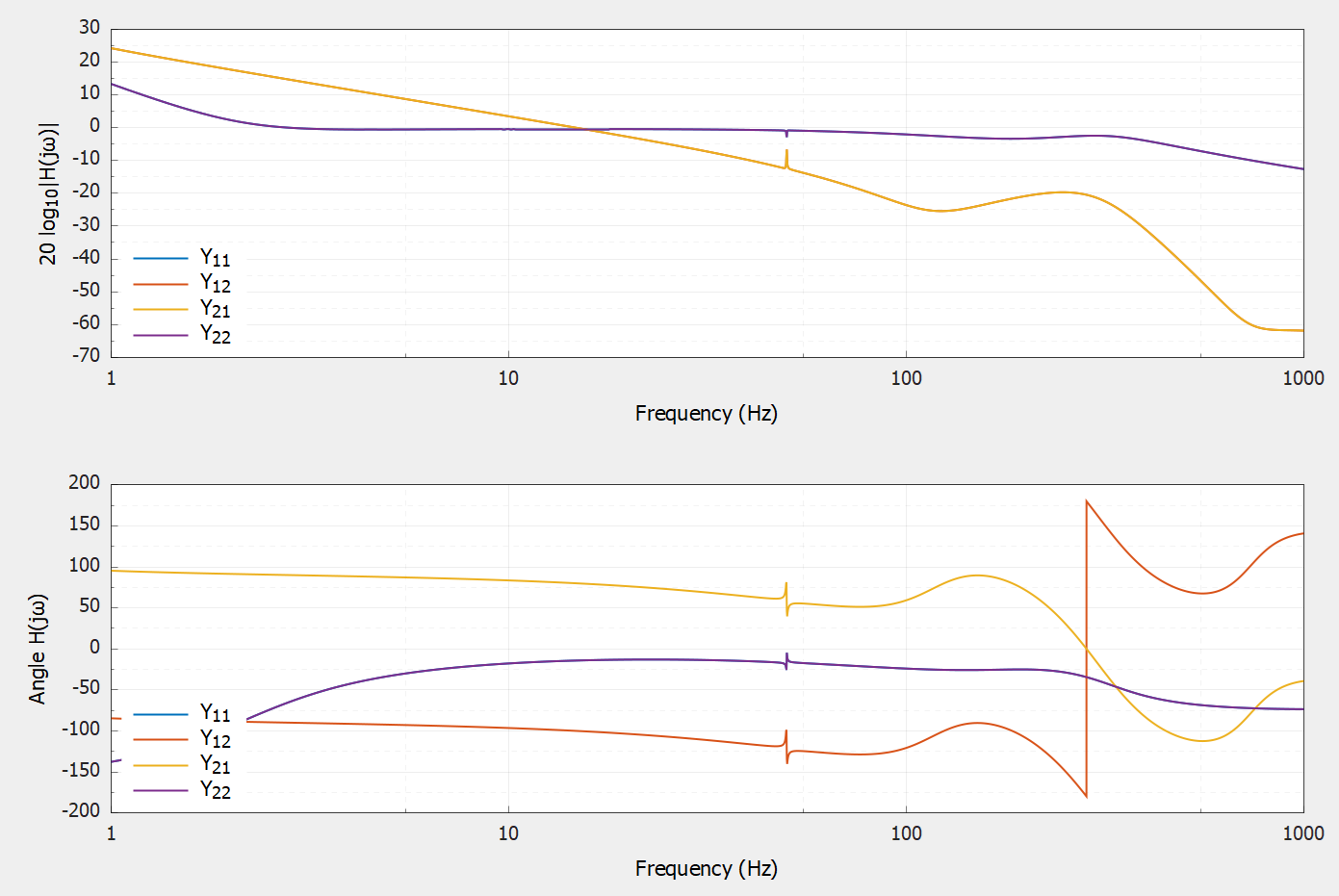
The equivalent total admittance is obtained as the parallel connection of the positive and negative sequences from RSC and GSC, like: \[\begin{equation} Y_{pn} = \begin{bmatrix} Y_{RSp} + Y_{GSp} & 0 \\ 0 & Y_{RSn} + Y_{GSn} \end{bmatrix}, \end{equation}\] and the dq admittance is estimated as: \[\begin{equation} Y_{dq} = \begin{bmatrix} 0.5 & 0.5 \\ -0.5j & 0.5j \end{bmatrix} \, Y_{pn} \, \begin{bmatrix} 1 & j \\ 1 & -j \end{bmatrix}. \end{equation}\]
Code Explanation
For detailed code information, see the Harmony manual.