Wind Turbine Type-4
Type-IV wind turbines (WT4), also known as full-converter wind turbines, employ a generator fully interfaced with the grid through a back-to-back power electronic converter. In this configuration, all generated power is processed by the converter, allowing complete decoupling between the generator and the grid. This enables wide-range variable-speed operation and flexible, independent control of active and reactive power. Owing to their superior grid-support capability and compliance with stringent grid codes, WT4 turbines are widely applied in weak-grid and offshore wind power systems, and are typically connected to the grid via a medium-voltage collector network and a substation transformer.
Mathematical Modeling
The typical structure of the type-4 WT is depicted in Figure 1.
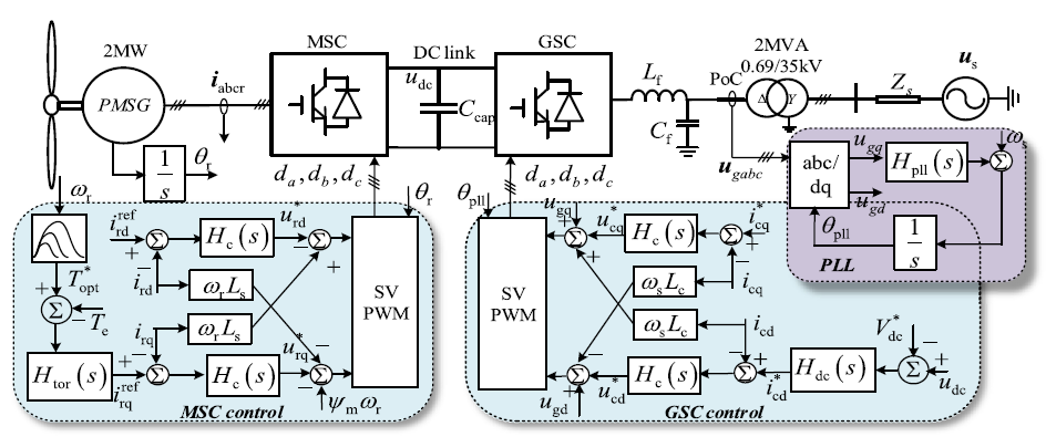
For the design of the model of WT type-4, the publication Arshad, Beik, Pallapati, et al. (2024) is used, with the corrections proposed in Arshad, Beik, Manzoor, et al. (2024) and He et al. (2025).
Namely, the WT is modeled by observing the dq-domain admittance looking into the GSC, which includes the PLL, current controller, output filter, delay, and a second-order input filter, as shown in Fig. Figure 2.
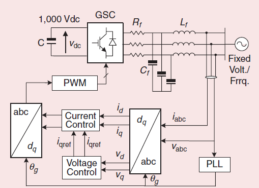
For such a model, the admittance can be calculated by taking into account:
\[\begin{equation} Z_f = R_f + s L_f, \end{equation}\]
\[\begin{equation} Y_{out} = \frac{1}{Z_f^2 + (\omega_g L_f)^2} \begin{bmatrix} Z_f & \omega_g L_f \\ -\omega_g L_f & Z_f \end{bmatrix}, \end{equation}\]
\[\begin{equation} G_{id} = - V_{dc} \, Y_{out}. \end{equation}\]
\[\begin{equation} H_{PLL} = \frac{K_{p,\mathrm{pll}} + \frac{K_{i,\mathrm{pll}}}{s}} {s + V_{d,\mathrm{ref}} \left(K_{p,\mathrm{pll}} + \frac{K_{i,\mathrm{pll}}}{s}\right)}, \end{equation}\]
\[\begin{equation} H^{d}_{PLL} = \begin{bmatrix} 0 & -M_{q0} H_{PLL} \\ 0 & M_{d0} H_{PLL} \end{bmatrix}, \qquad H^{i}_{PLL} = \begin{bmatrix} 0 & I_{q,\mathrm{ref}} H_{PLL} \\ 0 & -I_{d,\mathrm{ref}} H_{PLL} \end{bmatrix}. \end{equation}\]
\[\begin{equation} G_{mf} = \begin{bmatrix} \dfrac{\omega_n^2}{s^2 + 2 \zeta \omega_n s + \omega_n^2} & 0 \\ 0 & \dfrac{\omega_n^2}{s^2 + 2 \zeta \omega_n s + \omega_n^2} \end{bmatrix}, \end{equation}\]
\[\begin{equation} G_{del} = \begin{bmatrix} \dfrac{1 - 0.5 T_d s}{1 + 0.5 T_d s} & 0 \\ 0 & \dfrac{1 - 0.5 T_d s}{1 + 0.5 T_d s} \end{bmatrix}, \end{equation}\]
\[\begin{equation} G_{cc} = G_{dec} + G_{pi} = \begin{bmatrix} -\left(K_{p,cc} + \dfrac{K_{i,cc}}{s}\right) & -\dfrac{\omega_g L_f}{V_{dc}^2} \\ \dfrac{\omega_g L_f}{V_{dc}^2} & -\left(K_{p,cc} + \dfrac{K_{i,cc}}{s}\right) \end{bmatrix}, \end{equation}\]
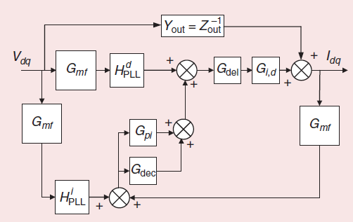
The admittance in the dq-frame is then calculated based on the flow-chart depicted in Figure 3: \[\begin{equation} Y_{dq} = (I + G_{del} G_{id} G_{cc} G_{mf})^{-1} \times (Y_{out} + G_{id} G_{del} (H^d_{PLL} + G_{cc} H^i_{PLL}) G_{mf} ). \end{equation}\]
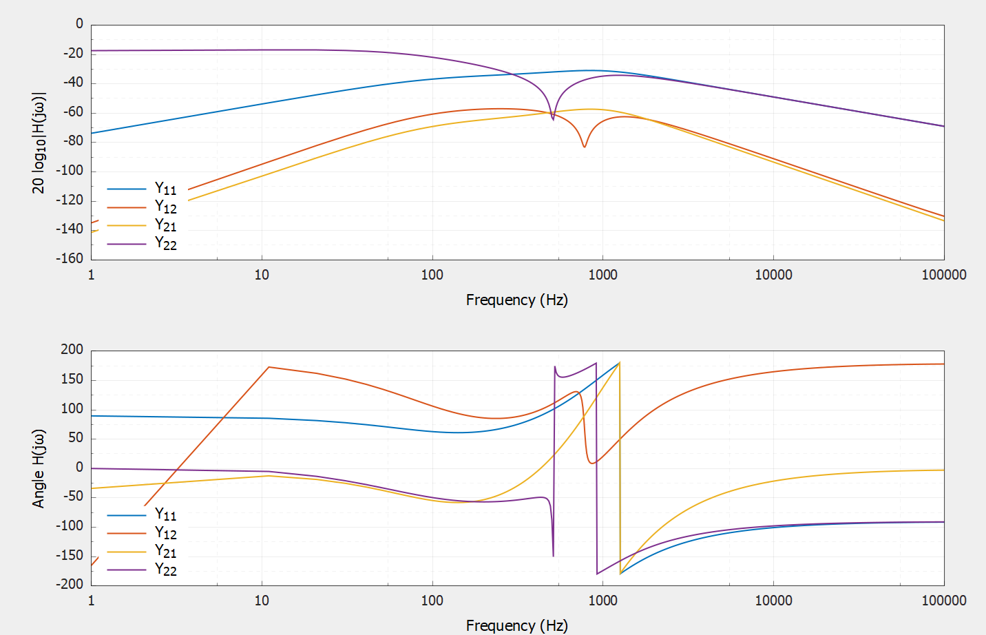
The results of the code execution in Harmony are available in Fig. Figure 4.
Code Explanation
For detailed code information, see the Harmony manual.