Generator

Tip

In power system analysis, synchronous generators are a fundamental component of energy generation. To model the interaction between the generator and the rest of the power network, admittance parameters (Y-parameters) are often used. The Y-parameters provide a relationship between the voltages and currents at the generator’s terminals and can be used in steady-state and dynamic analysis. This report presents the mathematical formulation of the Y-parameters for a synchronous generator, considering key electrical parameters such as field resistance, field inductance, direct-axis reactance, and field time constant.

Generator Model Parameters

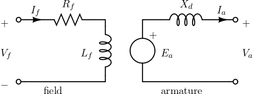
The generator’s behavior can be described using the following key parameters, as depicted in Figure 1:

• \(R_f\) - Field winding resistance;
• \(L_f\) - Field winding inductance;
• \(T_f\) - Field time constant;
• \(X_d\) - Direct-axis reactance;
• \(X_m\) - Mutual reactance;

These parameters represent the electrical characteristics of the synchronous machine and are used to derive the generator’s impedance and admittance.

Figure 1: Equivalent generator model.

Mathematical Modeling

In the frequency domain, the impedance of the generator can be described by its field impedance and direct-axis reactance. We form a two-port model with port 1 = stator direct axis and port 2 = field winding. Denote

\[\begin{equation} Z_f(s)=R_f+sL_f=R_f\big(1+sT_f\big),\qquad s=j\omega, \end{equation}\]

and let \(X_m=\omega M\) be the mutual reactance between stator and field windings. The impedance matrix of the coupled two-port is

\[\begin{equation} \mathbf{Z}(s)= \begin{bmatrix} jX_d & jX_m\\[4pt] jX_m & Z_f(s) \end{bmatrix}, \end{equation}\]

whose determinant is \(\Delta(s)=jX_d Z_f(s)+X_m^2\). The admittance matrix is the inverse \(\mathbf{Y}(s)=\mathbf{Z}^{-1}(s)\), which yields \[\begin{equation} \boxed{ \mathbf{Y}(s)=\frac{1}{\,jX_d Z_f(s)+X_m^2\,} \begin{bmatrix} Z_f(s) & -\,jX_m\\[6pt] -\,jX_m & jX_d \end{bmatrix}. } \end{equation}\]

Equivalently, the individual Y-parameters are \[\begin{equation} \begin{aligned} Y_{11}(s)&=\dfrac{R_f(1+sT_f)}{\,jX_d R_f(1+sT_f)+X_m^2\,},\\[6pt] Y_{12}(s)&=Y_{21}(s)=\dfrac{-\,jX_m}{\,jX_d R_f(1+sT_f)+X_m^2\,},\\[6pt] Y_{22}(s)&=\dfrac{jX_d}{\,jX_d R_f(1+sT_f)+X_m^2\,}. \end{aligned} \end{equation}\]

These expressions include the field first-order dynamics through \(T_f=L_f/R_f\) and are reciprocal \((Y_{12}=Y_{21})\).

Code Explanation

For detailed code information, see the Harmony manual.