This repository performs small-signal stability analysis of a two-machine power system, but with a twist: instead of plugging in numbers and computing eigenvalues, it keeps one physical parameter symbolic and derives a closed-form expression for each system eigenvalue and for its sensitivity.

Sweeping that symbolic parameter then answers a practical question:

As the parameter drifts away from its nominal value, does the inter-area oscillation mode stay well-damped? — i.e. how robust is POD the design?

In this walkthrough we keep the inertia ratio kH = H₂ / H₁ symbolic. We will:

Build the closed-loop state matrix of the system as a symbolic object.
Obtain a closed-form expression for the inter-area eigenvalue and its sensitivity in terms of kH.
Sweep kH (0.1 → 10) and plot how the mode moves and how its sensitivity behaves.

The full grid of configurations lives in scripts/generate_results.jl; here we isolate one configuration so each step is easy to follow.

1. Load the package

SymbolicES is this repository as a Julia package, so once the project environment is active a single using brings in the whole pipeline (symanalysis, the label dictionaries, …). We use CairoMakie to render publication-quality static figures.

using SymbolicES          # symanalysis(...) and friends
using Symbolics           # substitute, symbolic_to_float, @variables
using CairoMakie          # static, web-friendly figures
CairoMakie.activate!()

2. Pick one configuration

A configuration is a choice of what is symbolic and how the damping controller is designed:

Variable	Value	Meaning
`symvars`	`"kH"`	the inertia ratio H₂/H₁ is the symbolic parameter
`iinp`	`"p"`	POD input signal = line active power
`iout`	`"P"`	POD output = active-power injection
`jpod`	`3`	POD is connected at bus 3
`kbus`	`2`	the line power is measured towards bus 2

The nominal operating point is kH = 1 (equal inertias). We also tell the analysis that the feedback gain k is 0 at the nominal point — we are studying the open-loop modal sensitivity, i.e. the eigenvalue’s tendency to move the instant we start closing the loop.

@variables k kH      # k = feedback gain, kH = inertia ratio (both symbolic)

symvars = "kH"
iinp    = "p"
iout    = "P"
jpod    = 3
kbus    = 2

# Nominal point at which symbolic expressions are numerically checked.
dicCheck = Dict(k => 0.0 + 0im, kH => 1.0 + 0im)

# The inter-area mode we want to track (positive conjugate), ≈ 0.52 Hz.
target_eigenvalue = 0.0 + 3.27im

0.0 + 3.27im

3. Run the symbolic analysis

solve the AC power flow for data/bs_2area2gen_shiftbus3.m,
substitute kH into the generator inertia (H₂ = kH · H₁),
assemble the symbolic admittance matrix and the closed-loop state matrix Aex,
compute the four eigenvalues as expressions in kH (λres),
differentiate them to get the sensitivities ζ = dλ/dk.

c, λres, λcheck, ζ, ζcheck = symanalysis(symvars, dicCheck, iinp, iout, jpod, kbus)

symanalysis returns five dictionaries, each keyed by eigenvalue index 1:4:

λres — eigenvalues as symbolic expressions in kH,
λcheck — those same eigenvalues evaluated at the nominal point,
ζ — sensitivities dλ/dk as symbolic expressions in kH,
ζcheck — sensitivities evaluated at the nominal point,
c — the coefficients of the characteristic polynomial.

4. Find and inspect the inter-area mode

Of the four eigenvalues, we select the one whose nominal value sits closest to the target inter-area mode 0 + 3.27i.

eig_vals = collect(values(λcheck))
eig_keys = collect(keys(λcheck))
min_idx  = argmin(abs.(eig_vals .- target_eigenvalue))
mode     = eig_keys[min_idx]

println("Inter-area mode is eigenvalue #$mode")
println("Nominal value (kH = 1): ", eig_vals[min_idx])

Inter-area mode is eigenvalue #3
Nominal value (kH = 1): 3.2723739960829237994301791227986940302567795503603
67492257260671195715417822071im

This is the payoff of the symbolic approach — the eigenvalue is not a number, it is a formula in kH:

λ_expr = λres[mode]      # the inter-area eigenvalue as a function of kH

sqrt((1//2)*(-(141328907//15265061) - (91650935//32320881)*k + (18769229k) 
/ (4203737811kH) + (-701449819k) / (980085483kH) + (113511665k) / (83646305
73kH) - sqrt(-4((-294254609k) / (278333172kH) + (772077637k) / (730302300kH
) + (7597k) / (4348203795897kH) + (-46271036255k) / (160297722kH) + (146040
22891k) / (50593023kH) + 24341 / (54822661476804kH) + -162463 / (6938047129
572kH) + 2849808281 / (825616935kH) + -18480494489 / (19608888kH) + 6047242
6052 / (64164789kH) + -14704712767 / (4260097062kH)) + ((141328907//1526506
1) + (91650935//32320881)*k + (-1071719819k) / (879117408kH) + (701449819k)
 / (980085483kH) + (-113511665k) / (8364630573kH) + (-18769229k) / (4203737
811kH) + 236786951 / (635116170kH) + 117427333 / (1038498903kH) + 253153968
43 / (248688999kH) + -1315050353 / (220516101kH) + -3376258451 / (35719476k
H) + -411012143 / (1187264871kH))^2) + (1071719819k) / (879117408kH) + -236
786951 / (635116170kH) + -117427333 / (1038498903kH) + -25315396843 / (2486
88999kH) + 1315050353 / (220516101kH) + 3376258451 / (35719476kH) + 4110121
43 / (1187264871kH)))

and so is its sensitivity:

ζ_expr = ζ[mode]         # dλ/dk for the inter-area mode, as a function of kH

(-(91650935//32320881) + (4(7597 / (4348203795897kH) + -294254609 / (278333
172kH) + 14604022891 / (50593023kH) + 772077637 / (730302300kH) + -46271036
255 / (160297722kH)) - 2((9.25832572827583197997046981993717548852245005768
4014495585703850118908794403083 + 0.0im) + -411012143 / (1187264871kH) + 11
7427333 / (1038498903kH) + 25315396843 / (248688999kH) + -1315050353 / (220
516101kH) + -3376258451 / (35719476kH) + 236786951 / (635116170kH))*((91650
935//32320881) + -1071719819 / (879117408kH) + -18769229 / (4203737811kH) +
 701449819 / (980085483kH) + -113511665 / (8364630573kH))) / (2sqrt(-4(2434
1 / (54822661476804kH) + 60472426052 / (64164789kH) + -14704712767 / (42600
97062kH) + -162463 / (6938047129572kH) + -18480494489 / (19608888kH) + 2849
808281 / (825616935kH)) + ((9.258325728275831979970469819937175488522450057
684014495585703850118908794403083 + 0.0im) + -411012143 / (1187264871kH) + 
117427333 / (1038498903kH) + 25315396843 / (248688999kH) + -1315050353 / (2
20516101kH) + -3376258451 / (35719476kH) + 236786951 / (635116170kH))^2)) +
 113511665 / (8364630573kH) + 1071719819 / (879117408kH) + 18769229 / (4203
737811kH) + -701449819 / (980085483kH)) / (4sqrt((1//2)*((-9.25832572827583
1979970469819937175488522450057684014495585703850118908794403083 + 0.0im) -
 sqrt(-4(24341 / (54822661476804kH) + 60472426052 / (64164789kH) + -1470471
2767 / (4260097062kH) + -162463 / (6938047129572kH) + -18480494489 / (19608
888kH) + 2849808281 / (825616935kH)) + ((9.25832572827583197997046981993717
5488522450057684014495585703850118908794403083 + 0.0im) + -411012143 / (118
7264871kH) + 117427333 / (1038498903kH) + 25315396843 / (248688999kH) + -13
15050353 / (220516101kH) + -3376258451 / (35719476kH) + 236786951 / (635116
170kH))^2) + 3376258451 / (35719476kH) + 1315050353 / (220516101kH) + 41101
2143 / (1187264871kH) + -236786951 / (635116170kH) + -117427333 / (10384989
03kH) + -25315396843 / (248688999kH))))

5. Evaluate symbolic expressions

We now evaluate the two formulas over kH ∈ [0.1, 10].

kH_range = exp.(range(log(0.1), log(10); length = 100))   # 0.1 → 10, log-spaced

λ_trace = ComplexF64[]      # eigenvalue along the sweep
ζ_trace = ComplexF64[]      # sensitivity along the sweep

for v in kH_range
    sub = Dict(k => 0.01 + 0.0im, kH => v + 0.0im)

    λs = substitute(λ_expr, sub)
    ζs = substitute(ζ_expr, sub)

    push!(λ_trace, complex(Symbolics.symbolic_to_float(real(λs)),
                           Symbolics.symbolic_to_float(imag(λs))))
    push!(ζ_trace, complex(Symbolics.symbolic_to_float(real(ζs)),
                           Symbolics.symbolic_to_float(imag(ζs))))
end

println("swept $(length(kH_range)) values of kH")

swept 100 values of kH

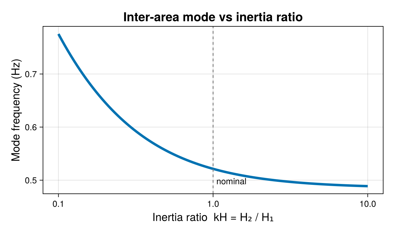
6. Inter-area mode frequency vs inertia ratio

freq_hz = imag.(λ_trace) ./ (2π)

fig1 = Figure(size = (640, 380))
ax1  = Axis(fig1[1, 1];
    xscale = log10,
    xlabel = "Inertia ratio  kH = H₂ / H₁",
    ylabel = "Mode frequency (Hz)",
    title  = "Inter-area mode vs inertia ratio",
    xlabelsize = 18, ylabelsize = 18, titlesize = 20,
    xticks = ([0.1, 1.0, 10.0], ["0.1", "1.0", "10.0"]),
)
lines!(ax1, kH_range, freq_hz; linewidth = 4, color = Makie.wong_colors()[1])
vlines!(ax1, [1.0]; color = :gray, linestyle = :dash)   # nominal point
text!(ax1, 1.05, minimum(freq_hz); text = "nominal", align = (:left, :bottom))

save("figures/example_frequency.png", fig1)
fig1

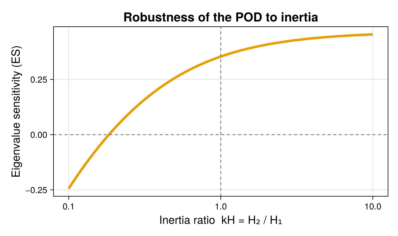
Inter-area mode frequency as the inertia ratio varies.

7. Eigenvalue sensitivity vs inertia ratio

This is the central result. The eigenvalue sensitivity (ES) measures how strongly the inter-area mode responds to the damping controller. We plot its imaginary part — the component that maps onto damping for this mode — against kH.

es = imag.(ζ_trace)

fig2 = Figure(size = (640, 380))
ax2  = Axis(fig2[1, 1];
    xscale = log10,
    xlabel = "Inertia ratio  kH = H₂ / H₁",
    ylabel = "Eigenvalue sensitivity (ES)",
    title  = "Robustness of the POD to inertia",
    xlabelsize = 18, ylabelsize = 18, titlesize = 20,
    xticks = ([0.1, 1.0, 10.0], ["0.1", "1.0", "10.0"]),
)
lines!(ax2, kH_range, es; linewidth = 4, color = Makie.wong_colors()[2])
hlines!(ax2, [0.0]; color = :gray, linestyle = :dash)
vlines!(ax2, [1.0]; color = :gray, linestyle = :dash)

save("figures/example_sensitivity.png", fig2)
fig2

Eigenvalue sensitivity of the inter-area mode vs inertia ratio — the robustness curve.