 WOLF-I
Multimachine Systems: Reference frame transformation
This post follows the method proposed in “Power System Stability and Control” by Prabha S. Kundur and Om P. Malik.
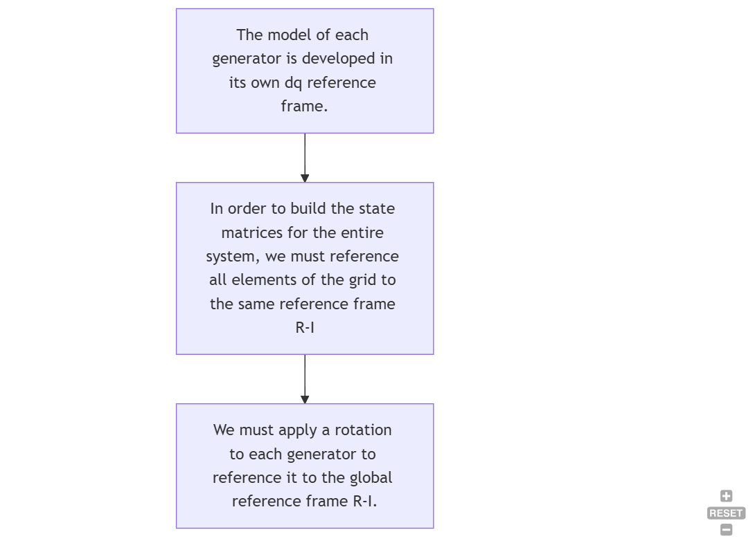
Building a multimachine linear system
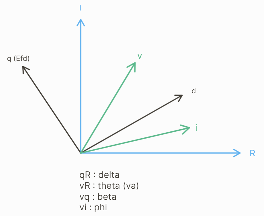
Reference frame transformation and associated angles between axes and variables
Linearizing:
\[\Delta i_{dq} = {\frac{dR}{d \delta}}|_{\delta = \delta_0}i_{IR0} \Delta x+R \Delta i_{IR} = {\frac{dR}{d \delta}}|_{\delta = \delta_0}{R^{-1}i_{dq}}_{0} \Delta x+R \Delta i_{IR} = t_i \Delta x + R \Delta i_{IR}\]Defining :
\[t_i = {\frac{dR}{d \delta}}|_{\delta = \delta_0}i_{IR0} =\begin{bmatrix}sin(\delta) && cos(\delta) \\ cos(\delta) && -sin(\delta)\end{bmatrix}\begin{bmatrix}-cos(\delta) && sin(\delta) \\ sin(\delta) && cos(\delta)\end{bmatrix} i_{dq0} = \begin{bmatrix}0 && i_{q0} && 0 && \cdots && 0 \\ 0 && -i_{d0} && 0 && \cdots && 0 \end{bmatrix}\]\([t_i] = 2 \times n\) , being \(n\) the number of state variables.
\[v_{dq} = R v_{IR} \rightarrow \begin{bmatrix} v_{d} \\ v_{q} \end{bmatrix} = \begin{bmatrix}-cos(\delta) && sin(\delta) \\ sin(\delta) && cos(\delta)\end{bmatrix} \begin{bmatrix} v_{I} \\ v_{R} \end{bmatrix}\]Linearizing :
\[\Delta v_{dq} = {\frac{dR}{d \delta}}|_{\delta = \delta_0}v_{IR0} \Delta x+R \Delta v_{IR} = {\frac{dR}{d \delta}}|_{\delta = \delta_0}{R^{-1}v_{dq}}_{0} \Delta x+R \Delta v_{IR} = t_v \Delta x + R \Delta v_{IR}\]Defining:
\[t_v = {\frac{dR}{d \delta}}|_{\delta = \delta_0}v_{IR0} =\begin{bmatrix}sin(\delta) && cos(\delta) \\ cos(\delta) && -sin(\delta)\end{bmatrix}\begin{bmatrix}-cos(\delta) && sin(\delta) \\ sin(\delta) && cos(\delta)\end{bmatrix} v_{dq0} = \begin{bmatrix}0 && v_{q0} && 0 && \cdots && 0 \\ 0 && -v_{d0} && 0 && \cdots && 0 \end{bmatrix}\]\([t_v] = 2 \times n\) being \(n\) the number of state variables
State space equations :
\[\Delta \dot{x}_i = A_i \Delta x_i + B_i \Delta v_{dq} \rightarrow \Delta \dot{x}_i = A_i \Delta x_i + B_i (t_v \Delta x + R \Delta v_{IR})\] \[\Delta i_{dq} = C_i \Delta x_i + D_i \Delta v_{dq} \rightarrow t_i \Delta x + R \Delta i_{IR} = C_i \Delta x_i + D_i (t_v \Delta x + R \Delta v_{IR})\] \[\rightarrow A = A_i + B_i t_v\] \[\rightarrow B = B_i R\] \[\rightarrow C = R^{-1}(C_i + D_i t_v - t_i)\] \[\rightarrow D = R^{-1}D_iR\]